
Index |
Last Chapter |
Next Chapter |
Simulando discitur
(By simulation learning is acquired)
- anon
Simulating nanoscale objects can be a powerful technique for understanding some of the mechanisms involved in cell function. It can be even more useful when combined with other computer-based techniques, such as 3-D modelling and image processing.
This chapter looks at how the nanosimulator can be used to improve modelling of cytoskeletal structures in plant cells, such as actin and tubulin filaments, and more complex structures such as plasmodesmata. A number of modelling techniques are used; image processing is done on raw electron micrographs, 3-D models are constructed based on these micrographs and other experimental data, and the resulting models are inserted into the nanosimulator as static structures, around which other objects (such as stain particles and antibodies) move and interact. The results of these simulations are taken from the nanosimulator and processed to produce 'Virtual Electron Micrographs' (VEMs) using physically reasonable models. These can then be compared with the original micrographs, to provide a check on the modelled data.
Part of the material in this chapter has been presented at the Third International Workshop on Basic and Applied Research in Plasmodesmal Biology, Zichron-Yakov, Israel 1996 under the title "Computer Assisted Analysis and Modelling of Plasmodesmata" (Betts, C., Conway, D., Radford, J., White, R.), and as "Virtual Electron Microscopy" (Betts, C., White, R.), at the 15th Australian Conference for Electron Microscopy, Hobart, Tasmania.
This section presents some of the raw material biological modellers work with. These 'Electron Micrographs' (or simply 'micrographs') are produced by a Transmission Electron Microscope (TEM), and show images of actin filaments and microtubules, as well as those of plasmodesmata. The images are taken from a variety of sources. Some were made using stained samples embedded in a thin sheet of resin, or sprayed onto a coated grid, or set in vitreous ice. All were taken at very high magnification, at close to the limit of a transmission electron microscope (other types of electron microscope offer higher magnification, but are unsuitable for many types of biological specimens).
These images show some standard micrographs of actin and tubulin:
 Figure 10.1 shows a typical
micrograph of negatively stained
actin from a coated grid. Note the
regularly spaced lines, caused by
the helical nature of actin
filaments. (1)
Figure 10.1 shows a typical
micrograph of negatively stained
actin from a coated grid. Note the
regularly spaced lines, caused by
the helical nature of actin
filaments. (1)
 Figure 10.2 shows a high
magnification image of a
microtubule in ice. Note the
regularities, again caused by the
structure's helical nature. (2)
Figure 10.2 shows a high
magnification image of a
microtubule in ice. Note the
regularities, again caused by the
structure's helical nature. (2)
Figure 10.3 shows another image of two microtubules, showing how microtubules appear within a cell. (3) The details are more difficult to see, and the ends are not visible in this image.
Plasmodesmata, the connectors between plant cells described in Chapter 2, are hard to examine under an electron microscope, due to difficulties in specimen preparation (primarily because it is difficult to cleave a plasmodesmata cleanly; usually the cleavage plane goes over or under the cylindrical structure). The following images show a transverse section and a longitudinal section.
Figure 10.4 shows a plasmodesma cross section. Notice the dark inner 'desmotubule', the (middle ring) plasma membrane, and the outer ring (probably caused by the opening funnel of the plasmodesmata). (4)
These raw micrographs, combined with other experimental results, are used by biologists in determining structure. However, due to practical difficulties with instruments, they are often far from perfect, as can be seen in the above images. At high magnification, a TEM micrograph becomes grainy and blurred, and there may be additional problems with contrast and photographic development.
Using computers it is possible to 'post-process' such images (as described in Chapter 3), to reduce the severity of these effects. For example, by stretching the grey-scale histogram of an image, the contrast can be improved, and by using an 'sharpening' filter, colour gradients can be intensified. To illustrate, this corrections were applied to figure 10.5 using the standard commercial PC package 'Paintshop Pro 5.0'), slightly improving its quality:
Histogram equalisation (summarised in Chapter 4) is a way of increasing the contrast of an image on a global basis, which can be very useful if an entire image is underexposed or overexposed. However, this technique often fails if the image contains both light and dark regions, but the individual regions are under- or over-exposed. It becomes more useful to do 'local histogram equalization (6), where each pixel is adjusted relative to its local area.
In order to enhance images of plasmodesmata such as figure 10.4, which feature very dark areas, especially in the desmotubule, a simple local histogram equalization algorithm was written as a plug-in to the 'Image Explorer' suite of image manipulation tools supplied by SGI. Applying this local histogram technique on figure 10.4 produced the following image:
There are many other possibilities for enhancing images. As a further example, a question that has often arisen regarding the large particles that are either embedded in the desmotubule (7), (8), or positioned between the desmotubule and the plasma membrane (9). Specifically it is unclear whether or not these particles are symmetrically arranged.
To help resolve this question, the image (Fig. 10.7) was processed using a polar Fourier transform (again, written as a plug-in for Explorer on the SGI), after which the angular high frequency components were dropped, using a low frequency angular bandpass filter (see Chapter 4 for a brief explanation of polar Fourier transform bandpass filtering).
The resulting image shows only the low frequency, i.e. rotationally repeated, components. We can see this in the image on the left, where the circular rings remain visible, but most of the other detail is either lost or reduced in intensity. Features closer to the centre are more accurately reproduced, since they subtend a relatively larger arc, and are thus more accurately described by the truncated Fourier spectrum.
The preceding image does not in fact show any strong evidence of rotational symmetry in the electron opaque (i.e. dark) areas in the desmotubule in the preceding image. Such rotational symmetry should express itself as a repeating rotational pattern in figure 10.9, but no such pattern is discernable. However a more intensive study on a large number of images using this and similar techniques would be needed before reaching any conclusion.
When the image, and even the processed image, does not give enough detail to fully determine the structure, other methods of investigation can be used to add further information. Usually however the electron micrograph at least places some general boundaries around the problem, by giving the rough dimensions of the structure, and possibly details about the regularity of the structure. These features, combined with available information on proteins present (derived from other experiments and analyses), can be used to create theoretical models that test the practicality of different arrangements of the proteins, membranes and other molecules making up biological structures.
A useful and long-established means of studying proteins and protein structures is the creation of 3-D models. Such 3-D models have ranged from toothpicks and plasticine to quite sophisticated works of machined wood and metal. Increasingly though, the ease with which computers can help researchers produce and manipulate 3-D models has led to the widespread adoption of computer-assisted modelling by researchers attempting to determine what protein conformations and arrangements are geometrically possible.
Despite the popularity of molecular modelling programs and 3-D CAD packages, it was not possible to find modelling software that could be easily used for this project, and as a result a simple 3-D modelling package was written from scratch, comprising of a number of separate viewing, scene creation, and processing utilities. This small package was able to read and save object definitions, output data in a variety of forms that could be used by other programs (including the nanosimulator), display results in real time using the Silicon Graphics hardware graphics library, and (most importantly) read in a mathematical description of object placement (especially helices). This last feature allowed the "single line" definition of thousands of separate objects making up a large helix, and was essential in creating some of the models described below.
All these features were available, and implemented to a far greater degree of sophistication, in other pre-existing packages, but unfortunately no single package combined all the features required. In order to maintain compatibility with future work, and the possibility of a better package appearing in the future, the modelling package was written to output data in both povray and wavefront formats, allowing other programs to also use the data.
In this thesis, most of the images are rendered in the 'Povray' raytracer, rather than using screen shots from the computer console, since this allows a great deal more detail to be displayed. To this end, minor details such as camera and illuminant positions are sometimes set manually to better frame the objects, as are material properties, such as whether the objects appear glossy or matte, and whether spheres are displayed as entirely discrete, or whether adjacent spheres are allowed to melt into each other. These finishing touches do not affect the geometry of the model, and are simply done to make the pictures clearer by giving the reader more visual cues to aid interpretation of the 3-D structure represented by the object. The reader should bear in mind that while the 3-D modeller utilities can model a wide variety of objects, such as cylinders, hollow cylinders, rectangular blocks etc., the nanosimulator itself is only capable of manipulating spheres.
Creating models of actin filaments and microtubules was a straightforward task. Models can easily be created by saving data from a nanosimulator session that had resulted in the growth of actin filaments or microtubules. This is normally done when the output of the nanosimulator is viewed and studied after the program is run.
Another way to create models of actin and tubulin assemblies is to model them as simple helices, twisting strands defined with mathematical precision. This can be an easier approach if it is necessary to precisely position an object. For example, if the object needs to be centred mathematically on the origin, this can still be accomplished with data saved from the nanosimulator, but usually requires the object to be manually re-positioned, since the object will have been moving about randomly within the simulation volume.
The models presented here were defined using simple mathematical helix definitions, and then rendered using povray. The model of actin in figure 10.10 is the standard model (10), however the microtubule model requires more explanation. Microtubules assemble into a number of different types of helix, and a given microtubule may even have a different structure within different regions (11).
These different structures are categorised by the number of protofilaments, or component longitudinal strands, within the microtubule. The most common variety (and the one modelled in previous examples by the nanosimulator) is the 13-protofilament model, but 14-protofilament microtubules are also quite common, and 12 and 15 protofilament microtubules also occur. As it is equally easy, using a mathematical description, to model any of these, a 12-protofilament microtubule based on the observational work of D.Chretién et al. (12) was chosen. The most obvious difference between these different microtubule types is that only the 13-start microtubule has straight protofilaments - in all other types the protofilaments form slowly twisting helices, as can be seen in figure 10.11 below. A final point to note is that in this particular representation no visual distinction is made between -tubulin and -tubulin.
Plasmodesmata, the connecting passages between cells in higher plants, were introduced in Chapter 2. The exact structure of plasmodesmata is not known for certain, although a number of similar models exist. A brief summary of some of the proposed models is given below:
This model (Fig. 10.12) shows the commonly accepted basic features of plasmodesmata; a tunnel between the cell walls lined with the plasma membrane, with a thin tube of endoplasmic reticulum (E.R.) passing through the centre, connecting, to some extent, the E.R of the adjacent cells. (13)
The Overall Model (Fig. 10.13) extends the standard model by postulating the existence of a number of globular proteins in the lumen between the desmotubule and the external plasma membrane sheath. (14)
This model (Fig. 10.14) modifies the standard model by including a role for a number of undetermined globular proteins embedded in the central desmotubule (or 'appressed endoplasmic reticulum protein complex', as it is referred to by the authors), and on the inner side of the plasma membrane sheath that lines the outer walls of the plasmodesmata, rather than in the lumen as above. (15), (16)
The Thomson model (Fig. 10.15), derived from observation of Tamarix salt glands, postulates particles in the lumen and embedded in the plasma membrane wall, in order to explain features found in freeze-fracture images. (17)
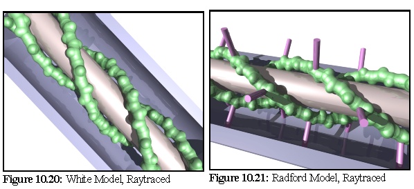
The White model (Fig. 10.18,10.20), based on the discovery of actin within plasmodesmata and TEM images showing "blobs" and "spiral blobs", postulates the existence of filamentous actin strands within the lumen, and raises the possibility of these being twisted around the central desmotubule. (18)
The Radford model (Fig. 10.19, 10.21) extends the White model to take into account the presence of myosin (an actin-associated motor protein) and TEM images showing apparent "spokes" within plasmodesmata. (19)
Four of the above models, namely the Ding, Overall, White, and Radford models, were modelled using the 3-D modelling tool. The modelling tool takes a short mathematical description of the models and renders them as a combination of rods, spheres, cylinders, cylindrical sheaths and helices of spheres. It is also capable of outputting their details in a variety of formats, for use by other programs, such as other real time viewers, ray tracers, and the nanosim program.
The fastest way of observing these models is by immediate rendering using the Silicon Graphics system. This also allows real time examination of the model, as the author's 3-D viewing program allows basic 3-D manipulation of viewpoint using a combination of mouse movement for rotation, and keyboard operation for panning the view point in and out.
The following images (Fig. 10.16 to10.19) are screen shots from the 3-D viewing program, showing the computer models constructed from four of the theories outlined above:
The above models can be very useful for real time viewing and examination, when an impression of the three dimensionality of the model can be obtained by real-time manipulations such as rotating the object, and by viewing from multiple angles. However, for still frame images it can be useful to render the objects in more detail using a ray tracer, to produce an image at a far greater resolution. This is important for high quality print reproduction, and it also provides a number of visual cues such as shadows, reflective effects, and improved shading, which may make the object appear more substantial and thus easier for viewers to interpret.
To this end, as part of the modelling program suite a simple conversion program was written to turn the mathematical description of models (such as those above) into povray raytracer files. This allowed the production of higher quality images such as these renditions of the White and Radford models below (Fig. 10.20, 10.21):
The nanosimulator was enhanced to allow it to read in pre-initialised structures, with the (current) limitation that such structures had to be static, and would not be able to move like other objects within the simulation. This was easily enforced within the program by giving such objects a diffusion coefficient of zero.
This allowed the input of models, such as those described above, into the nanosim program, where their interaction with other, motile, particles could be simulated. There are a great many possibilities for work combining pre-modelled structures with the nanosim program, even with the current limitation that such structures must be static.
Some such possibilities include:
To examine the usefulness of this technique, this last process of stain deposition will be examined and modelled in some detail.
An electron microscope works by passing a focussed beam of electrons through a sample of material, and displaying an image of the resultant attenuated beam. Since some parts of the specimen block the electron beam more than others, an image showing contrasting sections of the specimen can usually be obtained. How "electron opaque" an object is depends roughly on the size of its constituent atoms - light atoms are less likely to interact with the electron beam, while heavy atoms are more likely. So, for example, water is reasonably transparent under an electron microscope while heavy metals such as uranium are generally opaque.
Unfortunately, proteins and other biological molecules are, in general, made of fairly similar light atoms (carbon, hydrogen, nitrogen, oxygen) and so are comparatively transparent to the electron beam and difficult to distinguish from each other. In order to increase contrast between proteins (and also other organic molecules) in a biological specimen, the specimen is often stained with a heavy metal preparation that will preferentially bind to some, but not to all, of the material in the specimen.
After the specimen has been stained, and any excess stain removed, the specimen can be viewed with much greater contrast in the electron microscope. However stain deposition is not a well understood process, and artifacts can occur when stain is distributed unevenly.
A specimen for electron microscopy is usually prepared by embedding it in hard resin, to make the specimen physically stronger. This resin may impede the diffusion of stain particles, or prevent it altogether, depending on the exact resin and the stain used. Large stain particles, such as are used with antibody labelling techniques, usually cannot penetrate the resinous substrate, and will only stain, (or 'label') the part of the specimen that is exposed outside the resin. Smaller stain particles on the other hand may be able to penetrate the resin, although they may take some time to do so.
The nanosim program can simulate the movement of the stain particles around a computer model of a 3-D proteinaceous structure (such as those shown in the previous section), with the model being optionally embedded, or only partially protruding from, an impenetrable resinous substrate. A solution of stain particles is modelled as drifting over the surface of the structure, with some of the stain particles binding to the structure. How the substrate is modelled, or whether it is modelled at all, depends on the type and size of stain and the permeability of the resin being simulated.
This method of stain deposition is shown on a variety of cell structures: filamentous actin, microtubules, and one of the plasmodesmata models. By also modelling an impermeable substrate, and applying the stain particles from the 'top' of the model, it is possible to also simulate any uneven distribution of stain particles over a sample.
As mentioned previously, the nanoscale simulator is capable of reading in a pre-existing structure at start up. However, since the nanosim program is only capable (at the moment) of working with objects composed of spheres, it was necessary to modify the 3-D modelling program to output the existing models in a form that the nanoscale simulator could read. The difficulty here is that the 3-D modelling program deals with complex surfaces, such as rotationally symmetric parabolic or trigonometric surfaces, as well as rectangular blocks, cones, cylinders and such like, in addition to spheres.
This was resolved by saving such non-spherical objects as a large number of component spheres. The method is similar to the well-known computer technique of modelling 3-D objects as a vast number of small, cubical building blocks known as 'voxels' (21). This increased the computational load on the simulator, since it greatly multiplied the number of objects the simulator had to consider, but the population remained within manageable limits.
Creating a model suitable for the nanoscale simulator was thus a two stage process. Firstly the model was constructed using the 3-D modelling program, and then the model was converted into a vast number of spheres for use by the nanoscale simulator. A small change to the 3-D modelling program enabled the different components of the high level description to be given names, which were set to correspond to defined protein types in the nanoscale simulator's 'protein dynamic description file', or '.pddf' file.
The stain particles were modelled as very small, very mobile, very easily bound particles that started in a layer above the 3-D structure and substrate, and diffused downwards. The particles were assumed to bind to everything except each other. While the actual heavy metal ions that form most common stains are in fact minute on the scale of the simulator, the actual particles were made somewhat larger, to reflect their associated solvation layer water molecules (which slow their movement).
In order to simulate the differential binding of the stain to different parts of the model, the number of binding sites for the different proteinaceous components of the model was varied, or their strength altered. Thus proteins known to stain heavily were given a large number of binding sites, whereas proteins that are harder to stain were given fewer and/or weaker binding sites.
After a period of time representing the staining process, unbound stain particles were removed, corresponding to the washing out of unbound stain particles that occurs during specimen preparation. The resulting simulator state was saved to an output file suitable for the povray raytracer.
Figure 10.23 shows the stain having been deposited on the microtubule model in figure 10.22. The model is not shown actually in the sea of stain particles, since the picture would appear as almost entirely black. Only the stain particles that have been bound to the surface of the model are included in the picture.
The type of stain shown above involves a very large number of very small stain particles. A different type of stain is used in antibody staining, where smaller numbers of very large and specialised stain particles are used instead. Antibody staining is usually a two stage process. The primary antibody (a protein that binds very specifically to another protein) is used to bind to the target protein in the specimen. Because the antibody is a protein itself, it is transparent to electrons (or 'electron lucent'). As the purpose of staining the specimen is to create electron opaque regions, a further stage of staining is done with a secondary antibody to the first antibody. The secondary antibody is conjugated to an electron opaque metal particle. This complex attaches to the bound antibody creating the final stain marker, which indicates the presence of the particular protein species the primary antibody was targeting.
An attempt was made to model this on a cross-section of a plasmodesmata model, showing the action of antibodies staining for actin.
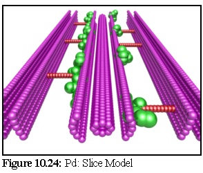
The model used in this example is the Radford Model (Fig. 10.19,10.21). To make our simulation as realistic is possible, the model is imbedded in a 'virtual resin', by making the bottom portion of the simulation field impermeable to stain particles, and only the thin exposed surface layer is modelled, giving effectively a thin slice through the model as an active region.
Notice the way the plasmodesma cross-section (especially the various membrane bi-layers) has been remodelled as a large number of spheres (Fig. 10.24). Also observe the many overlapping spheres. Although different objects within the nanosimulator cannot overlap, the spheres making up the components of one particular object in the nanosimulator can (this was shown earlier with actin in Chapter 7). In the current simulation this idea is extended. All static objects are allowed to overlap, and no collision checks are performed between two static objects, only between objects where at least one object is motile.
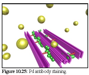
Figure 10.25 shows the primary antibodies, starting above the plasmodesmal section, ready to diffuse (the substrate layer has been made transparent in this image).
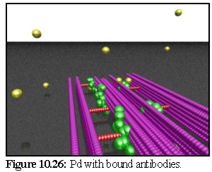 In figure 10.26 a period of time has passed:
some primary antibodies are free while a few
(visible at the rear of the image) have bound
to the model below. In this example the
model is imbedded in impenetrable resin,
beyond which the stain particles cannot
move. (The static spheres are not so
restricted, and in fact the model is very
slightly embedded in the resin).
In figure 10.26 a period of time has passed:
some primary antibodies are free while a few
(visible at the rear of the image) have bound
to the model below. In this example the
model is imbedded in impenetrable resin,
beyond which the stain particles cannot
move. (The static spheres are not so
restricted, and in fact the model is very
slightly embedded in the resin).
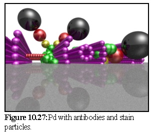
In figure 10.27 the simulation is finished, and the unbound particles have been removed. Second stage staining by the metallic particle (black) and the secondary antibody(red) has not been fully simulated; they have simply been added on to the primary antibody (yellow) in an opposite direction to the link (i.e. perfect antibody recognition has been assumed).
A classic problem with modelling cellular structures on a computer is in comparing them with images of the real structures taken from electron microscopy. The computer models are usually too precise and uncluttered, whereas the real structure suffers from the difficulties of staining, contamination, resin embedding, damage during preparation and the limitations of the imaging technique used.
In a real laboratory staining exercise, after the specimen has been exposed to the stain for a period, the excess stain is washed off, leaving behind only the stain particles that have bound to the specimen. The program emulates this by removing all unbound stain particles after the simulation of deposition has been completed.
Having obtained our model results from the nanoscale simulator in the previous section of stain deposition or antibody motion, a 'virtual electron micrograph' (or VEM) is produced using a ray tracing program that represents stain particles as being very dark, and the rest of the structure and substrate as being translucent. The result is an image of the computer model as it might appear to a 'virtual electron microscope', and this enables the researcher to compare their model, to some extent, with experimental data.
This simple approach (i.e. using a raytracing program) to electron microscope modelling is possible due to relative translucency of thin biological specimens. If a denser object was being simulated (such as a mineral sample), it would be necessary to model the multiple interactions of each electron with the sample as the electrons bounced through the material, using more complex techniques such as Monte-Carlo simulation, which uses a randomiser to model a large number of electron paths. However, since the chance of multiple sample interaction with a thin biological sample is very low, this complexity can be ignored, and a single pass model can be used. This can be done easily using a normal ray-tracing program with no perspective adjustments (i.e. parallel rays).
An investigation of the basic premise of this idea was attempted before proceeding with the full stain deposition simulation. A simple computer model, which represented stain particles as black dots on an otherwise invisible model was constructed. This simple model did not include any substrate. It produced a simple image, which was then post-processed to reproduce some of the visual flaws of an electron microscope. There are a number of such flaws that could be simulated.
This can be simulated using a small scale blur filter, similar to those in Chapter 2, or by a Fourier transform that removes high frequency components.
This can be simulated using a noise generator, i.e. a simple algorithm that randomly brightens and darkens areas of the image. The simplest example is a point noise generator, that randomly adds black and white dots to an image.
Astigmatism can be simulated by a global transformation function over the whole image, using a shear transformation matrix. This is a standard technique (22), where every pixel in an image is repositioned using the formula p' = Tp, where p' is the new position of the pixel, p the original position, and T the transformation matrix:
 Formula 10.1: 2-D Vector Transformation.
x', y' - the new position of the pixel
a,b,c,d - elements of the transformation matrix
x, y - the original position of the pixel
When the matrix T is the identity matrix![]() the position of the pixels does not change. If
instead the values of a and d are set to some other value than 1, while b and c remain zero (i.e.
the position of the pixels does not change. If
instead the values of a and d are set to some other value than 1, while b and c remain zero (i.e.
![]() ), a linear shear, or skew, results that emulates the effect of astigmatism.
), a linear shear, or skew, results that emulates the effect of astigmatism.
The hexagonal grain pattern of a real photographic image could be simulated by averaging hexagonal areas, and re-rendering as black circles with a radius giving the same overall darkness to the previously averaged area. The method is very similar to the ray tracing technique of over sampling, used to reduce aliasing, when an image is generated (sampled) at a higher resolution than the final image, each pixel in the final image being an average of several samples (23). It is possible to do the same with hexagonal pixels, as illustrated below.
Since the model includes no attempt at random stain patterning, it produces very obvious (and unrealistic) regularities in the image. Lines and patterns of points (exacerbated by perspective effects) can be seen which do not appear in real TEM micrographs. Real TEMs do of course have some regularities, and these are very important for researchers determining structure, but the initial images below are far more regular than in real images.
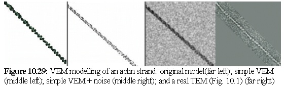
Actin was the first structure that was considered. Figure 10.29 shows an actin filament at various stages of image processing - the image second from the right is the final 'virtual electron micrograph'.
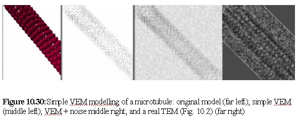
In the same manner, a virtual micrograph of a microtubule was constructed. Note the pronounced regularity of the staining pattern.
While the above can be a useful method, since it is very quick to produce such an image from a 3-D model, it suffers from not simulating the stain deposition very accurately, which gives rise to the regularities and Moiré patterns shown above. A more complete approach is to use the results from the previous section that modelled in more detail the deposition of stain.
Taking the results from the nanosimulator, the stain particles are rendered as being a dark translucent grey (corresponding to the electron opaque nature of stain), while the model itself is rendered as a far lighter translucent grey (corresponding to the electron lucent nature of most proteins), as was the substrate. To imitate the operation of an electron microscope, all refraction effects were turned off in the ray tracer, so that the 'light rays' the ray tracer simulates would go straight through all the model materials without any prismatic bending or refraction. In addition, the raytracer's rays were made to run parallel (or with less than one minute of arc of divergence), thus removing any perspective distortion, and again modelling the essentially parallel nature of the electron beam in a TEM.
This method was used on well known structures first, to establish its basic validity, and then on some less well known structures. The first structure simulated in this way was that of a 12-filament microtubule, after which the same technique was used on a hypothetical model of plasmodesmal structure.
These images show the original microtubule model, and again show the resultant 'virtually stained' image from a small, resin-infiltrating stain particle.
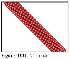
Figure 10.31 is the Original Model (From Fig. 10.22).
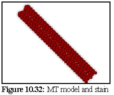 The Model covered with stain, displayed without perspective, and with stain particles
displayed as 150 picometer spheres is shown in figure 10.32 (see also figure 10.23). The stain
particles are assumed to be able to attach to any of 25 equivalent binding sites on the tubulin
dimers, although geometry will prevent all of these sites being bound to (i.e. other tubulin
dimers obscure some of these attachment sites).
The Model covered with stain, displayed without perspective, and with stain particles
displayed as 150 picometer spheres is shown in figure 10.32 (see also figure 10.23). The stain
particles are assumed to be able to attach to any of 25 equivalent binding sites on the tubulin
dimers, although geometry will prevent all of these sites being bound to (i.e. other tubulin
dimers obscure some of these attachment sites).

Figure 10.33 shows a rendering of the VEM, without any post processing.
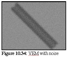
Figure 10.34 shows the VEM with random shot noise to simulate TEM imperfections. In this
technique, a random 10% of pixels are set (with equal probability) to either completely black
or completely white.
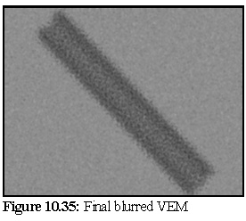
In other words, the value of each pixel is determined by placing the above filter over the image, centred on the pixel being blurred, and the resultant pixel is the average of all the neighbouring pixels.
Other more elaborate masks were also used, but gave much the same effect, while the above filter has the advantage of speed, as it can be implemented as a simple summation of all the neighbourhood values, followed by a single division by 25.
 For comparison, here is an inset of figure 10.2, rotated
to the same angle as above. As can be seen, the above
model fails to reproduce the regularities of the real
TEM, probably due to inadequacies in the staining
model being used, which assumed an even distribution
of stain attachment sites on the modelled tubulin dimers
(these can be compared with the unstained VEMs
presented later in this chapter).
For comparison, here is an inset of figure 10.2, rotated
to the same angle as above. As can be seen, the above
model fails to reproduce the regularities of the real
TEM, probably due to inadequacies in the staining
model being used, which assumed an even distribution
of stain attachment sites on the modelled tubulin dimers
(these can be compared with the unstained VEMs
presented later in this chapter).
An added factor is that the above model is a twisting, 12-filament microtubule, while the above picture is presumably the more common 13-filament type, however the difference is not actually that great; images of 12-filament microtubules show a slight change along their lengths as their filaments spiral, but preserve the basic features of this photograph.
(Further study of microtubules, done without simulated staining, is done after the next section)
Next, a hypothesised plasmodesmata model (the Radford model, cf Fig. 10.19,10.21) was examined. This particular model includes a number of twisted actin strands (green), as well as some unusually small myosin proteins (red) and a number of membranes representing the desmotubule (the inner cylinder) and the outer plasma membrane of the plasmodesmata (the outer skin of the model). The labelling of this model by a primary antibody, followed by a secondary antibody with an associated gold particle, is shown in figures 10.24 to 10.27.
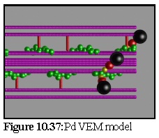
Figure 10.37 shows the plasmodesma, labelled by a number of small antibody particles. It is identical with the model shown in figure 10.27, after the stain deposition modelling process (Fig. 10.24 to 10.26) has occurred. This image is simply taken from above, with no perspective.
Figure10.38 is the raw VEM, showing the plasmodesma embedded in resin, being labelled by three large antibody particles. Note that the unstained proteinaceous components are comparatively faint next to the completely black antibody heads, representing the gold spheres used in this type of antibody label.
Finally, figure10.39 shows the VEM with the same shot noise and blurring used previously (i.e. 10% of pixels set evenly to black or white, followed by a 5�5 averaging filter).
This can be compared to a real image (Fig. 10.40) of antibody labelled plasmodesma (the plasmodesmata is running vertically, at a slight angle, and the position of the stain particles are marked by the black indicating arrows). (24) This image is slightly misleading however, since in addition to antibody labelling, it has also been post-stained with a traditional heavy metal stain, as was modelled in the microtubule example previously.
 As can be seen the images are similar only in broad outline.
The grainy appearance of this particular real TEM
(probably caused by stain clumping , and possibly some
degree of photographic development artifacts) is modelled
poorly by pixel level shot noise: a more advanced approach
would be required, possibly some variation of the
hexagonal 'photographic film graininess' approach,
combined with a modelling of the secondary staining
process.
As can be seen the images are similar only in broad outline.
The grainy appearance of this particular real TEM
(probably caused by stain clumping , and possibly some
degree of photographic development artifacts) is modelled
poorly by pixel level shot noise: a more advanced approach
would be required, possibly some variation of the
hexagonal 'photographic film graininess' approach,
combined with a modelling of the secondary staining
process.
While modelling stain deposition is a challenging problem, useful results can be obtained (in real microscopy as well as virtual) without stain. While the contrast is fainter, very clean specimens such as in-vitro assembled microtubules can still produce excellent results.
Some exceptional work on in-vitro assembled microtubules has been done by Denise Chrétien of the Laboratoire de Biologie Structurale in France, using highly purified tubulin polymerising in thin films, which are then rapidly frozen and examined on a cryogenic stage in an electron microscope (25), (26). In particular the work suggests some interesting features of assembling microtubule ends, indicating that they are curved and splayed out, as is shown by the following image (Fig. 10.41) (27). Chrétien et al. interpret these (and other) images to suggest that microtubule growth occurs when an initially flat sheet grows and curls into a closed microtubule.
To demonstrate further the use of virtual electron microscopy, a static model (not from the simulator) is constructed displaying some of the curved end features postulated by Chrétien et al. (i.e. a double-curvature growth spike, but not the flattening effect, which is shown in the upper diagram within figure 10.41.
The model was constructed in povray using the file shown in Appendix G. It was then blurred, and noise added, in order to simulate the imperfections of electron microscopy.

Images 10.42-10.44 show the modelled microtubule, with the curved, open end. The first image (Fig. 10.42) is a perspective view of the model, showing the nature of the doubly curved open end. The second image (10.43) is an orthographic view of the model side on. The third image (10.44) shows the model (again with an orthographic view) within a randomly positioned cloud of dimers (statically modelled, rather than simulated) .
Simulating an electron micrograph using the model from figure.10.44 produces the image shown in figure 10.45. Note the unrealistically crisp resolution of the image. The image is produced using a light source directly behind the model, and by making the dimers translucent. The dimers are also shrunk slightly, to represent the more electron opaque core of the protein (hence they appear as double spheres rather than dumbbells).
In figure 10.46 a Gaussian blur of radius 4 pixels is applied (the image is 1280x1024 pixels in size). A small amount of pixel level noise is added to give a slight graininess to the image.
As can be seen, the VEM faithfully reproduces a number of the features of the real micrograph (Fig.10.47), such as the banding along the body of the tube, and the relative intensity of those bands.
However, the features of the growth tip are not identical, which is a useful result, as it indicates that the model used (a curved, tapered section of the normal microtubule with the same cross-sectional curvature) is probably not what realistically occurs in nature (which is likely to be a thinner spike with fewer protofilaments (28)).
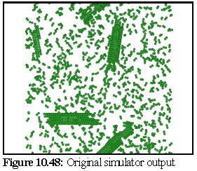
The VEM image retains rather more contrast and resolution than the original, but although it could be degraded further there is probably no need. The close modelling of striations and the relative strengths of the striations, especially in the closed body of the microtubule, is an excellent example of the strength of the technique. VEMs of this sort (i.e. without staining) can be made relatively quickly, probably in real time, and are a useful adjunct for the protein modeller. To demonstrate, the following images (10.48,10.49, and 10.50) of microtubule fragments are taken from a simulated microtubule construction run from Chapter 8:
Creating a virtual micrograph of a computer model is simply another way of looking at a model - it neither proves, nor disproves, the model's validity. It may however suggest that a certain model is more accurate than another, by showing that the protein structure corresponding to a given model would be more likely to produce the TEM images observed than the protein structure corresponding to another model.
A difficulty with this method is that the actual process whereby stain particles bond to proteins is not entirely understood. In modelled structures containing unknown or unidentified proteins, it can be particularly difficult to decide how well stain particles will bind to a particular component of the model. For example, when a very regular stain deposition was assumed (e.g. Fig. 10.30) the staining was unnaturally regular, which created visual artifacts. When a more random staining model was assumed (e.g. Fig. 10.35) there was possibly not enough regularity to properly model the staining process, since the degree of regularity found in real TEM micrographs was not observed (e.g. Fig. 10.2).
A further complication, shown by figures 10.39 and 10.40, is that the simple staining model used does not handle the interaction between stain particles, which sometimes results in stain clumping into electron opaque aggregates, that can again give an image a grainy appearance.
The usefulness of the technique is shown in figures 10.41 to 10.50, which demonstrate how virtual electron microscopy can support a structure hypothesis, by confirming the observed banding and edge density effects shown in microtubule TEMs.
This chapter shows how the principle of the nanosimulator can be extended to model the interaction of particles with static structures. It illustrates one way that static structures could be incorporated into the nanosimulator, and then showed the nanosimulator in operation, using both static and dynamic objects, and links between these two types of object.
This chapter has demonstrated some of the wider possibilities for the nanosimulator and how it can complement traditional image processing techniques. A number of image processing techniques were investigated, and the results used to improve raw TEM images.
The concept of virtual electron microscopy was explored, where 3-D models of biological structures are algorithmically manipulated in a way that emulates the physical processes involved in obtaining and developing a transmission electron micrograph. A brief investigation of the defects and artifacts introduced in the physical micrograph was made, with some suggestions for future work.
Extending the idea of the virtual micrograph, an investigation was made of how the staining process used for electron micrograph specimen preparation might be modelled using the nanosimulator. Preliminary results were obtained that showed promise, however it was also shown that there was need for a more sophisticated model of staining.
The illustration of staining is only one of many possibilities for modelling nanoscale structures. Modelling diffusion and structured growth will also be feasible using the existing program, and doubtless many other types of simulated experiments will also be possible.
Index |
Last Chapter |
Next Chapter |
1. Image from Alberts, B. et al, Molecular Biology of the Cell, (1994), Garland Publishing Inc., New York, Fig. 16-2, p789
2. (Detail from) Image from Alberts, B. et al, Molecular Biology of the Cell, (1994), Garland Publishing Inc., New York, Fig. 16-49, p789
3. Image courtesy J. Radford, Monash University Dept. Biological Sciences.
4. Image courtesy J. Radford, Monash University Dept. Biological Sciences.
5. Image courtesy J.Radford, Monash University Dept. Biological Sciences.
6. Gonzalez, R.C. and Wintz, P., Digital Image Processing, (2nd ed. 1987), Addison-Wesley Publishing Company Inc., Reading Massachusetts, Chap 4.2.4 pp 158-160
7. Ding, B., Turgeon, R. and Parthasarathy, M.V. (1992) Substructure of freeze-substituted plasmodesmata Protoplasma, Vol 169, pp 28-41
8. Botha,C.E.J., Hartley, B.J. and Cross, R.H.M., The Ultrastructure and Computer-enhanced Digital Image Analysis of Plasmodesmata at the Kranz Mesophyll-Bundle Sheath Interface of Themeda triandra var. imberbis (Retz) A.Camus in Conventionally-fixed Leaf Blades, Ann. Bot. Vol 72: pp255-261
9. Overall, R.L., Wolfe,J. and Gunning, B.E.S., (1982) Intercellular Communication in Azolla Roots: I. Ultrastructure of Plasmodesmata Protoplasma, Vol 111, pp 134-150
10. The actin model is now well understood - see any standard reference such as Amos, L.A; Amos, W.B. Molecules of the Cytoskeleton, (1991) Guilford Press, New York
11. D.Chrétien et al., Lattice Defects in Microtubules: Protofilament Numbers Vary Within Individual Microtubules, (1992) J. Cell Bio., Vol 117, pp 1031-1040
12. Ibid.
13. Alberts, B. et al. op.cit. p962
14. Gunning B.E.S. and Overall R.L., Plasmodesmata and Cell-to-Cell Transport in Plants (1983), BioScience Vol 33 No 4 pp 260-265
15. Ding B., et al, Substructure of freeze substituted plasmodesmata, (1992) Protoplasma Vol 169, pp 28-41.
16. Illustration from Lucus et al, Tansley Review No. 58, Plasmodesmata and the supracellular nature of plants, (1993) New Phytol, Vol 125, pp 435-476, based on Ding B., et al.(1992) above.
17. Thomson W.W. and Platt-Aloia, K. (1985), The Ultrastructure of the Plasmodesmata of the Salt Glands of Tamarix as revealed by Transmission and Freeze-Fracture Electron Microscopy Protoplasma Vol 125, pp 12-23
18. White R., personal communication.
19. Radford, J., Ultrastructure of Plasmodesmata, (1994) Honours Thesis, University of Sydney, Dept Biological Sciences.
20. Alberts, B. et al, Molecular Biology of the Cell, (1994), Garland Publishing Inc., New York, pp807-808
21. Voxels are a well known 3D graphics technique, mentioned in most good textbooks - e.g. Hearn, D. and Baker, M.P., Computer Graphics (2nd ed.)(1997) Prentice Hall, Sydney, Australia, pp 360-362.
22. Ibid. pp 203-205, 423
23. This is a common ray tracing technique; e.g. see Cook, R.L., Stochastic Sampling and Distributed Ray Tracing, Chapter 5 of 'An Introduction to Ray Tracing', edited by Glassner, A.S., 1989, Academic Press Ltd., San Diego, CA.
24. White, R. et al. (1994) op. cit.
25. Chrétien, D., Meteoz, F., Verde, F., Karsenti, E., & Wade, R.H., (1992) Lattice Defects in Microtubules: Protofilament Numbers Vary Within Individual Microtubules, J. Cell Biol., Vol 117, No. 5., pp 1031-1040
26. Chrétien, D. (1991) Apports del al cryomicroscopie électronique à l'étude de microtubules assemblés in vitro, Ph.D. Thesis, Université Joseph Fourier, Grenoble, France (cited ibid)
27. Chrétien, D., Fuller, D., and Karsenti, E. (1995), Structure of Growing Microtubule Ends: two-Dimensional Sheets Close Into Tubes at Variable Rates, J. Cell. Biol., Vol 129, No.5, June 1995, pp 1311-1328
28. Jánosi, I.M, Chrétien, D., Flyvbjerg, H. (1998), Modeling elastic properties of microtubule tips and walls, Eur Biophys J., Vol 27, pp 501-513