Since the simulation is mathematically complex, a number of utility classes are used to simplify the tasks
of vector and matrix arithmetic. Using the C++ facility to overload operators, it becomes possible to
write many vector and matrix equations in an intuitive form that considerably simplifies the appearance
of code.
There are two utility classes used in the program: a point class and a matrix class. They perform vector
and matrix arithmetic, and allow expressions such as X=A+B, X=A-B, X=A*B and
X=A^B where
the '+' and '-' operators are normal addition and subtraction, while the '*' operator is used for vector
cross product and, somewhat counter intuitively, the '^' operator is used for the vector dot product (for
programmatic reasons it is impossible in C++ to use the '.' character for this purpose). These functions
are defined for various appropriate combinations of scalars, vectors and matrices. Other vector
operations are defined to allow various common tasks such as rotation around a fixed axis, the
calculation of magnitudes, division by reals, and so on.
Finally, an external mathematical function provided by Professor Chris Wallace of the Department of
Computer Science and Software Engineering at Monash University is used to generate the fast pseudo-random
Gaussian numbers which are widely used throughout the program.
An overseer is necessary to co-ordinate the activities of all these separate classes. This co-ordinating
object (there is only one) interprets the command line arguments of the user, starts the parsing of the
.pddf initialisation parameter file, and initialises the required monomers to start the simulation.
Once this initial housekeeping is finished, the co-ordinator runs the program loop, cycling through the
sequence of movement, binding and breaking. During this process it calls the objects responsible for
visual output, and directly logs numerical data to a data log file.
Before the program can simulate an environment, it must know what the environmental conditions are,
and what proteins (or generic objects) it is simulating. While the general rules of behaviour for objects,
such as their Brownian motion behaviour and the way they join together, are immutable and held in
program code, exact details such as the size of the simulation field, the number of monomers in the
simulation, and the exact properties of those monomers are set by configuration files and command line
parameters.
Once the relevant information has been obtained by the program, it must correctly initialise the
simulation's data structures, placing monomers in their starting positions, initialising the grid of 3-D
'cells' in which the monomers move, initialising the mathematical look-up tables used for collision
calculations, and generally 'setting up the pieces' for the simulation.
Some features of the simulation are independent of the protein data files, and should be easily
changeable by the user. These are handled at the command line, and include details such as the molarity
of the solution (i.e. the number of objects to be simulated), the size of the simulation field in
nanometres, and details of what data to output and how often. Most importantly, it is at the command
line that one specifies which .pddf file to use.
It is not, strictly speaking, necessary to explicitly specify all these details. The program uses default
values for any unspecified parameter, which is useful for rapid testing and prototyping of .pddf files.
These default values can easily be changed within the program but, as an example, typical values are:
- a concentration of 5 molar;
- a total field size of 256 nanometres cubed; and
- the .pddf file 'info.pddf'.
Reading Data from the .pddf file
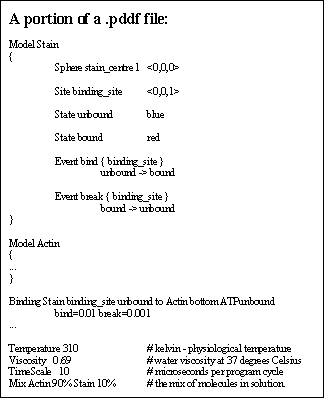 The amount of data necessary to describe the behaviour of a protein monomer are far greater than can
be reasonably entered at the command line. As a result, small text files that can be written by human
users, are used instead (see 'Appendix C; Protein Dynamic Description Files' for a full language
description.)
These 'protein dynamic description files' or
'.pddf files' contain all the data necessary to
describe (in the simulation) the dynamic
behaviour of the monomers. Details such as the
general shape of the monomer, the binding sites,
states of the monomer, and the events that
trigger those states must be listed. Optional
details such as the mass and diffusion constants
of the protein can also be included, although
the program will estimate these if they are
unknown or not provided.
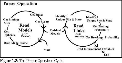
The program parses these .pddf files, storing the
data in internal data structures that are similar,
but not identical to, the elements described in
the .pddf files.
In order to build these data structures, the
parser works through the .pddf file, recording
data in a fixed sequence (Fig.6.3): first it reads
the data for each individual protein species, then
it reads data about the binding linkages, and
their chance of breaking, between monomers.
Next it reads the environmental variables (which
specify details such as the temperature and viscosity of the simulation environment), the timestep for
each simulation cycle, and finally the mixture ratio for the different protein species (if multiple types of
monomers are present).
Initialising the Environment
Once this data set has been read into the program, the co-ordinator works out details such as how many
monomers should be created and how large the simulation field should be.
Next the 3-D data grid is initialised with the correct field size - this involves initialising each grid cell
with the correct 3-D co-ordinates.
Then the monomers are created, and given (uniformly distributed) random positions within the
simulation field. They start the simulation in their initial state, with no linkages to other monomers. The
temperature and viscosity details have already been used to calculate the diffusivity of the monomers if
this was not explicitly stated, and this is converted to a 'root mean square position delta' which
describes
how far the monomer moves, on average, each
time step.
(See Chapter 5 for details of this calculation).
Finally,
environmental conditions are recorded explicitly
and
independently of the various monomer species, for
use in
later calculating the diffusivity of the various
polymers.
Special
Conditions and Work in Progress
 An
addition to the functionality of the program is the
ability to
define starting positions for the monomers.
Among
other benefits, this allows simulation of diffusion
from high-concentration regions to low-concentration regions. An obvious extension of this procedure
would be to allow complete simulation states, including linked polymers, to be read in as starting
conditions, but this has not yet been completed.
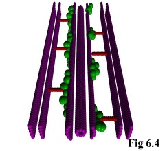
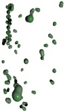
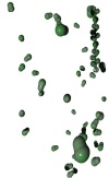
As an addition to the functionality of the program, it is possible to include static objects in the
simulation (e.g. Fig. 6.4), thus allowing the simulation of particles moving through restricted areas, such
as channels, holes, or simply past large structures. This is done by allowing the user to define monomer
species with a diffusivity of zero, i.e. which do not move.
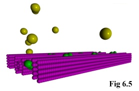
The program treats these as special cases, and fixes them immutably in
space. The actual objects can then be read in using the above method of
pre-defined positions, after which they can interact normally with other,
freely moving, objects (Fig. 6.5).
Program Actions: The Moves
The basic classes and objects give a static picture of the program. This next section describes their
dynamic nature - how they behave within the simulation.
The Co-ordinator's Cycle:
At the top level, the co-ordinator works through the initialisation steps outlined above before entering a
continuous cycle. But most of these initialisation functions are carried out by other objects; the only
functions directly performed by the co-ordinator are those of initialising the virtual environment and
logging numeric data.
Once the simulation is running normally, the co-ordinator's role is simply to prompt various objects into
performing their actions on cue. Aside from this, the co-ordinator is also responsible for numeric data
logging.
Moving Monomers and Dimers
Monomers and polymers are usually required to move during the simulation. This involves both linear
displacement and rotational motion.
'Linear' Motion
'Linear' motion is used in the sense of the non-rotational change in position of objects - however, since
they are moving in a Brownian manner, the actual path taken by the objects is likely to be far from
linear. All objects, both monomers and polymers, have a diffusivity which enables the RMS change in
position to be calculated (as described in the previous chapter). Because the particles are travelling in a
Brownian manner with a very small 'step-length' their full path need not be simulated. Instead the
particles are moved directly to a randomly determined position using this RMS change in position.
Although the linear motion of large, non-spherical molecules (such as actin polymers) should be slightly
different due to their irregular shape, the program currently does not handle this. Very large molecules
in fact move very slowly on the scale of the simulation, so this inaccuracy has negligible effect.
The program does, however, take into account the approximate shape of the polymer when calculating
the raw diffusion constant. It does this by approximating the shape of the polymer with an ellipsoid of
the same moment of inertia, and using that ellipsoid in the diffusion constant equations outlined in the
previous chapter. Hence, while strict directionality is not modelled, the overall diffusion behaviour is
reasonably accurate.
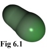
After completing a movement cycle, the program checks that no particles are overlapping, and moves
them apart to 'just touching' if this has occurred. This is done by considering the component spheres
making up the overlapping objects (cf Fig. 6.1). In order of greatest overlap, each sphere is separated
from it's neighbour by moving their centres directly apart along the line connecting their centres, and the
process is repeated if necessary until the objects are entirely separate. Algorithm 6.1. summarizes this
process.

It is theoretically possible that this process could end in an infinite loop (although this has never been
observed), so an error check is included as a fail-safe. If the process repeats more than 20 times, the
position of one of the objects is set to a random location within the simulation field.
As an alternative to the above, a more elaborate algorithm using a bounding box for each polymer, and
moving the centroid of each polymer away until the bounding boxes just touched would avoid the
looping problem, although care would have to be taken in the case of polymers with irregular geometry
not to leave unnaturally large spaces between the objects.
Approximating Rotational Motion
Rotational motion for monomers is quite straightforward: at the time scales used by the simulation
(usually cycles are on the order of microseconds) it is assumed that the monomers will tumble so much
as to assume an essentially random orientation at the end of each cycle. Hence, after each cycle they are
set to point in a completely random direction. This approximation holds well for timesteps > 1 s and
monomer sizes < 10 nm.
However, as explained in the previous chapter, a more elaborate approximation is used for rotational
motion in polymers, which is assumed to be energetically similar to linear motion. In a further
approximation, the Brownian nature of the linear motion is extended to rotational motion, and again the
distribution is assumed to be the same.
Hence no rotational momentum is calculated, instead the rotating body is assumed to be bumped by
innumerable smaller particles, eventually arriving at a final position every time step, in a result based on
a Gaussian distribution. This Gaussian distribution is set by the program to be energetically identical to
that of the linear motion equation. In this case however allowance is made for the shape of the polymer,
and the moment of inertia is used in calculating the Gaussian distribution along each axis.
A further constraint requires that the user has entered the .pddf files in such a way that the co-ordinates
for the primary axes of the MOI (moment of inertia) coincide with the Cartesian axes of the .pddf file.
The reason here is simply computational efficiency; in the absence of a more detailed model of rotation
there seems to be no reason to correct the slight error caused by approximating the MOI to the co-ordinate axes rather than calculating the full MOI. tensor.
Note that the fact the MOI is known and calculated during
movement makes it possible for the modelling of the linear motion of
the polymer to be improved, if a suitable model for the Brownian
motion of irregular objects becomes available.
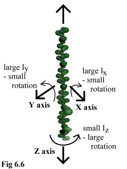
The final result of these approximations, then, is that large polymers
behave in a manner that is mechanically reasonable. Long thin
polymers such as actin strands (e.g. Fig. 6.6) or microtubules may
spin easily around their major axis, but will not deviate far in rotating
around their minor axes, whereas globular polymers (such as viral
capsid assemblies) will tumble equally in all directions. The full
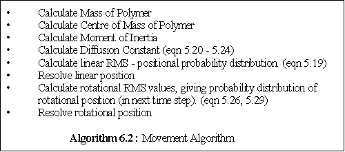
movement algorithm is given by algorithm 6.2.
Boundary Conditions
One of the most challenging programming tasks was, surprisingly,
the correct handling of boundary conditions within the simulation.
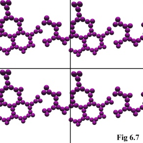
As explained in the previous chapter, the model uses a tessellated
boundary condition to simulate an infinite space for the physical
objects to move within (Fig. 6.7). In practice, this simply means that
objects leaving one side of the cubical simulation volume are
'wrapped-around', appearing immediately through the opposite side
of the simulation.
This is a trivial programming task for single monomers, although
some special handling is required during interaction testing and so
forth (detailed below), when the centre of the monomer may be on
one side of the simulation volume while some of the monomer's
component spheres are on the other side.
However it becomes a far more significant task for polymers, because they will frequently have
monomers on two sides of the cubical simulation field. In fact, it is not unknown for a polymer in a
corner of the simulation field to have monomers existing in all eight corners of the simulation cube
simultaneously. This makes it essential to 'normalise' the position of these border polymers when doing
linear or rotational movement. This 'normalisation' simply involves moving the polymer into the
positive octant of the Cartesian co-ordinate system (i.e. all co-ordinates in the +x,+y and +z region of
space) before manipulating it, and then 'de-normalising' the polymer and moving it and its constituent
monomers back into the simulation field proper. To put it another way, 'normalisation' is enlarging the
positive octant so that the entire polymer simulation space falls within it. It should be emphasised that
this process is done only for polymers straddling the simulation boundaries, which are usually a very
small minority of all the polymers in the simulation.
While this is not too arduous, the programming difficulty is increased when handling unusual situations
such as the joining of two polymers, and can even become inconvenient in more mundane tasks such as
the adding or shedding of a monomer from a polymer. For example, it is necessary to normalise the
polymer before the moment of inertia and diffusion constant are calculated. These boundary conditions
must also be borne in mind when checking for errors or unusual conditions (e.g. for polymers joining
across the simulation field boundary), a fact that can make such checks substantially more
computationally expensive.
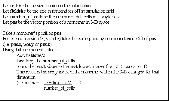
Populating the Data Grid
As mentioned previously, the program uses a 3-D 'bucket' system to store the monomers (either free, or
bound within polymers) within the system for swift access (Algorithm 6.3 describes the bucket access
system). The simulation space is divided up into a grid of cubical cells, each cell of which maintains a
list of all the monomers within its borders. The grid is a 3-D array, which is indexed by an x, y and z
integer index.
Every time the monomers move, either freely or as part of polymers, this data grid must be reset, and all
the monomers registered with the appropriate data cell. Since the simulation field is centred on the
origin (i.e. it extends equally into all eight octants), some minor adjustment is needed to allocate a
monomer to the correct data cell.
Summary
of
Object
Movement
The
program's
treatment
of
molecules
may
be
summarized as follows.
Molecules:
- move in a Brownian manner;
- move in discrete jumps;
- always rotate to a random orientation;
- have polymer rotation approximated in a physically reasonable manner;
- have boundary conditions that are allowed for;
- populate a 3-D data grid; and
- have collision checks made after movement.
Object Interaction
After they have moved, the objects must be checked to see if they have come close enough to interact.
The actual calculation of whether a protein in solution is going to bind to another would be quite
arduous, and would presumably require detailed treatment of the protein's solvation sphere, the surface
charge distribution, the geometry and nature of binding sites, and so on. Fortunately all these factors
can be reduced to a single probability - the probability that, if and when the two monomers collide, they
bind. (In fact, the technique is slightly more subtle than this - see the section on 'calculating binding
probabilities' below.)
The first step then in calculating interactions is to see whether the monomers will collide. As explained
in the previous chapter, due to Brownian motion this is not as simple as it might first appear.
Collision Probabilities
In classical frictionless Newtonian conditions, particles continue on their way until they are acted upon
by a force, such as collision with another particle. In such conditions, determining whether two particles
collide is, at least in theory, purely a matter of deterministic mathematics.
In this simulation, however, the number of collisions is so immense that such methods are infeasible.
Instead, we must consider the problem of how to calculate the probability of two particles, each moving
in a Brownian manner, colliding. This is done by numeric simulation, (as explained in the previous
chapter, and in Appendix A). In the program the values from such a pre-calculated numerical simulation
are used to calculate (given the position, sizes and RMS movement values of two monomers) the chance
of collision during the next time step.
Each monomer is tested against its neighbours in its own, and in adjoining, grid cells. This, in turn,
provides an upper bound on the length of the time step. As the time step increases, the range of each
particle per time step also increases (as the square root of the time step). If the time step is too large,
then the simulation becomes inaccurate because a particle may interact with others that are more than
one grid cell distant - a possibility the program does not check. As a result, for strict accuracy, the time
step should be such that the size of a grid cell is larger than three standard deviations of monomer
movement (i.e. 3 times the RMS change in position).
In practice this constraint can probably be relaxed without great consequence, because the method used
to calculate binding probabilities will adjust these binding probabilities to a slightly higher value to
compensate for the lost opportunities for more distant interactions. Nonetheless, time steps leading to
one standard deviation monomer movements of more than one grid cell width should almost certainly be
avoided, because this will remove the program's ability to accurately simulate local concentration
gradients and may affect the accretion rate of large polymers.
Object Binding
When monomers are found to have collided, the chance of binding for the two closest available (i.e. not
already in use) binding sites on the two monomers is checked. (This use of the closest sites may require
binding probabilities to be adjusted if some sites thus become more geometrically likely to link up than
others). At this stage, the chance that binding would occur is found using the data originally read in
from the .pddf file, and the monomers bind with that probability. A randomiser is used to generate a
number from zero to one, and if it is greater than the required probability as specified by the user, then
binding commences.
A relatively complex procedure is required to simulate binding. Three situations can occur: either both
monomers are unbound and floating free; or either one of the monomers is part of an existing polymer;
or both monomers are part of existing polymers.
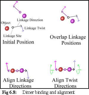
Binding Free Objects
The first condition that must be satisfied is that the
objects are oriented and positioned with respect to
each other (Fig. 6.8). This is done by moving the
objects (if one is bound, only the free object is
moved) so that the two objects' linkage sites are
coincident, and their 'direction' vectors are exactly
anti-parallel. The objects are then rotated so that
their 'twist' vectors coincide.
If both monomers are free, a new polymer object is
created to store the data of the union. First a
polymer object of mass zero, with no objects, is
created. One monomer, and then the other, is
added to the new polymer, causing the polymer to
update its internal list of 'owned' monomers.
At the same time the physical properties of the polymer are updated: the polymer acquires the summed
mass of its constituent monomers, the centroid (the 'centre of gravity') of the polymer is calculated, and
from that the moment of inertia is calculated using the parallel axis theorem to sum the moments of the
constituent dimers. Finally, using this moment of inertia and the aggregate mass, the diffusion constant
of the new polymer is calculated in the manner outlined in the previous chapter. Before any of these
calculations are done the monomers are 'normalised', if necessary, to avoid the difficulties of calculating
these constants in a polymer that spans the simulation field boundary.
To summarise, when free monomers bind together:
- the monomers are physically aligned according to their binding links;
- a new polymer is created;
- the monomers are registered with this polymer;
- the polymer mass is calculated;
- the centroid is calculated;
- the moment of inertia is calculated; and
- the diffusion constant is calculated.
Binding a Free Monomer and a Bound Monomer
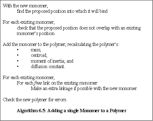
If one of the monomers is bound, the procedure is slightly different. Firstly, a check is performed to
make sure that the position into which the new object will fit is not already taken. This is done by
iterating through all the monomers already bound to the polymer, and making sure that no physical
conflict exists between the proposed position of the newly binding monomer, and the positions of the
existing monomers.
Secondly, the new monomer is added, and the polymer properties updated as outlined above. Finally,
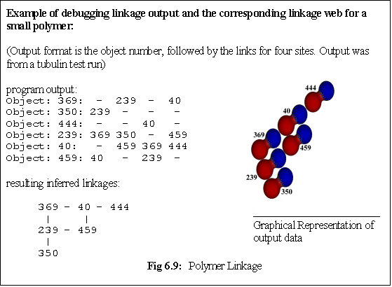
further checks are made to see whether any additional links are possible - i.e. whether the new monomer
has 'slotted into' a position that is adjoined by multiple bound monomers (Fig. 6.9, algorithm 6.5).
While the polymer does not explicitly record the linkages its constituent monomers make, it does
initiate these checks for extra 'cross-links' between its 'owned' dimers. The algorithm used is not
optimal - it simply interrogates every monomer in turn, asking it whether it is adjacent to the new
monomer and in a position to bind it. If this is the case a new link is created. This can lead to quite a
complex set of links within a polymer (Fig. 6.9), which must be correctly maintained as monomers are
added and, more importantly, as they are deleted.
After the monomer is added, more checking is carried out to ensure that the polymer does not enter an
illegal state, e.g. with bound monomers believing they are attached to other monomers that are now
free, or (somehow) monomers overlapping each other within the polymer. Fortunately, although such
checking is vital during program development, it is usually unnecessary when the program is stable and
running normally.
Merging Two Polymers
The most complex situation is when two colliding monomers are already attached to others, and hence
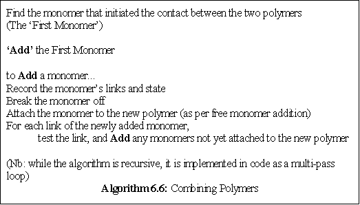
two polymers must be joined. The algorithm used takes a record of every monomer in the smaller
polymer, along with its links and state. The monomer which initiated the binding, is bound first. Next
that monomer's old neighbours are 'brought across', being removed from the old polymer and attached
to the new polymer, and then rebound with the same links that they had previously, and then
(recursively) all the neighbours that they had are brought across, and so on. As each monomer is added
it is tested to see if it physically 'fits' into the new polymer (i.e. that there are no obscuring pre-existing
monomers), and if it does not fit it simply returns to the pool of free monomers in the correct state
(algorithm 6.6). While this may seem a little artificial, in fact it seldom occurs that two polymers come
together (although this can still be a significant assembly path), and even more seldom does it happen
that they have 'jagged edges' that break off during assembly. After all the monomers have been brought
across, the old polymer (now empty of monomers) is destroyed.
It is theoretically possible that this algorithm could lead to two misshaped polymers overlapping, and the
first polymer 'stealing' a single monomer, and 'unzipping' the remaining polymer completely. While this
could occur if the polymers were irregularly shaped, it represents a pathological case that should occur
very rarely.
Unbinding
In every cycle after all new bindings have been completed, all polymers check to see if any of their
constituent monomers break away. (The probability of this happening is set by the user in the .pddf
file.) If they do, the monomer must undergo internal checking to see if this event triggers a change in
state. Meanwhile the polymer must recalculate its physical characteristics, and check for any orphaned
monomers that no longer have links connecting themselves to the bulk of the polymer. Furthermore, the
polymer must check that it still exists - if the polymer is reduced to a single monomer, it loses its raison
d'être and frees the remaining monomer before deleting itself.
The probability of a multiply-bound monomer unbinding must be calculated, depending on the program
options used (the methods are explained in more detail in Chapter 5). In the .pddf file the user specifies
whether the probability of multiply bound objects is:
- zero : they cannot break off;
- the multiplicative sum of all bound links; or
- the 'order of magnitude' heuristic, which divides the smallest link probability by ten for
each extra link (see algorithm 6.7).

State Changes and
Random Events
When monomers bind or break away, their internal state machine checks to see if the particular binding
or breaking event was significant enough to change the state of the monomer. It should be emphasised
that it is quite possible for an object to have only one 'state' - for example the properties of a stain
particle might not change depending on whether or not it is bound (although it would probably change
valence). Many proteins however undergo relatively complex state cycles, from a free phosphorylated
state, through to various bound states, and finally back to a free unphosphorylated state, from which
they may recover over time.
The state machine not only checks every binding and breaking event to see if the state changes, but also
whether the current state is unstable - i.e. whether there is a random chance of decaying into a different
state. Such a random event can be used to simulate the stochastic rephosphorylation of an
unphosphorylated protein, or the dephosphorylation of a recently bound protein.
The Program Cycle: Playing the Game
Having examined the individual components of the program, the overall functioning of the simulator
should now be fairly clear. The Co-ordinating Object runs the following execution path (Fig. 6.10):
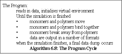
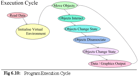 Data are read in from the user in the form of command line arguments and .pddf initialisation files. The
virtual environment is then set up: memory is allocated, data structures initialised and objects created.
After this is done, the co-ordinator enters a repeating cycle of object movement and interactions that
either runs for a fixed length of time, or until interrupted by the user (algorithm 6.8).
The accessing of objects is done in separate ways depending on context. The co-ordinator maintains a
complete list of all objects, and this is used during the movement phase to move all unbound monomers.
Since monomers are never created or destroyed during the program execution, this is an efficient way to
access them. Polymers are continually being created and destroyed, so they are tracked using a linked
list. During movement this linked list is iterated through, and each polymer moved. During collision
prevention (a sub-phase occurring immediately after movement) and the object interaction phase, the
objects are accessed via the 3-D grid cell array, with all grid cells being consecutively searched for
objects, and when an object is found, adjacent cells are checked for occupancy and consequent
interaction. For disassociation, objects in polymers are again searched by linked list. Objects being
checked for a random state change within polymers are also checked from the polymer linked list, while
free objects are accessed via the co-ordinator array of all objects.
State changes occurring due to binding and breaking occur immediately, while state changes due to
random events (e.g. rephosphorylation) occur after the breakage phase.
At the end of the cycle comes data output. Usually the program does not output data every cycle.
Depending on user parameters the program will output numerical data logs on a regular basis (the
default is 200 cycles). These numerical data logs indicate the number of objects, how many objects are
free and how many in polymers, a break-down of how many objects are in which states, the size
distribution of aggregates, and track the changes over time in selected individual polymers.
In addition the program may save visual and geometric data files. If directed to, it will save a geometric
data file suitable for a raytracer (e.g. every 10,000 cycles), and can even save a quick 'snapshot' of the
graphics window as a separate option (e.g. every 1,000 cycles). These 'snapshots' can be useful for
debugging an unattended run, or quickly creating animations, because they do not require the overhead
of running the ray-tracer.
At the end of the program's execution the program outputs all its normal data sets, and some further
data. This includes a speed index (number of object cycles per second achieved), and a detailed list of
the final size distribution of aggregates.
A Special Mode: Working Out the Probabilities
An obvious difficulty with the nanosimulator program is how to obtain the probabilities for the binding
and breaking away of monomers to and from polymers. Ideally these numbers would be obtained from
a detailed understanding of the protein structure and its binding sites. Useful approximates however,
can be inferred from studies of bulk properties (i.e. by observing how much raw material polymerises in
a solution, combined with a knowledge of how many individual polymers exist). Such experimental
studies can give rise to raw 'on and off' rates for monomers. (4)
Translating these into program terms is still non-trivial. To convert the 'off-rate' into a value that can
be used by the program is quite straightforward - if monomers break off the tip of a polymer at the rate
of five a second, we can simply multiply by our time step (for illustration, say 1 ms) to find the
'breakage probability' for the link (in this case p(breakage) = 5 * .001 = 0.005 per time step).
To translate the 'on rate' (which depends on concentration) into a binding probability for a single
dimer, it is necessary to know how many collisions occur in one time step.
To discover this, the simulator is run in a special test mode, in which no binding actually takes place.
Instead the number of collisions with a stationary test monomer (representing the growth tip of a
polymer) is recorded. Using this number, and modifying it if necessary to take into account the number
of binding sites, it is possible to work out the binding probability.
For example, if in a 1 ms time step a monomer with two symmetric binding sites experiences, on
average, 10 collisions, and the on rate is 12 monomers/second, we would find the binding probability as
P(binding) = (12*.001)/10 = 0.0012 per time step.
Development Notes
The nanosimulator computer program was written in conjunction with a number of other programs,
some written by the author and some available as freeware from other sources.
Development Environment and Portability
The computer language chosen for development was C++, because it is a high-level, object-oriented
language that still compiles to fast machine-level instructions. The development took place on a series
of Silicon Graphics machines, and was finally finished on an SGI O2 R10000. The final program runs
under SGI Irix 6.3 (a Unix variant), and primarily used the 'gnu' freeware C++ compiler 'g++'. It uses
the older SGI 'gl' graphics library for real-time output.
In an effort at portability, a version was created without the SGI-specific code, and compiled under the
other main Unix operating system variant, System V, running on a DEC station. Since the main thrust of
the program is numerical simulation, there is good reason to believe it could be compiled with ease on
other platforms (such as PCs), but the lower performance of such machines means that this has not yet
been attempted.
While real-time graphical output is not currently available on non-SGI systems (an 'OpenGL' version is
planned for the future, and will run on a wide range of systems including PCs), the program saves
'Povray' format ray-tracer files (details of this program are given below).
Related Programs
In addition to the simulator, a number of other programs were developed for this project. Firstly, a 3-D
modelling utility program capable of taking a mathematical description of objects and returning it in a
number of formats was written. Secondly, a small collision testing program (described below) was put
together. Thirdly, testing the program required some test- bench and debugging software to be put
together. Fourthly, a 3-D object viewing program was written to allow fast 3-D manipulation of
geometric data files, and a subset of this program was later incorporated directly into the nanosim
program itself.
A number of externally written programs were used, the most important of which was the Povray ray-tracing program. Povray is a popular ray-tracer developed by a large community of graphics
programmers; it is freely available at the web site http://www.povray.com, as is documentation, a
number of examples, and some other utility programs. The Povray ray-tracer is available on all major
platforms (Unix, Macintosh, PC, Amiga, and others). Also used in general image preparation was the
'xv' Unix graphic file viewing utility.
Finally, the image processing described later in this thesis was largely done using the SGI Explorer
package, which provided a framework for image processing modules, as well as a number of pre-written
basic image processing functions (such as Fourier transforms and filter functions). The extended image
processing modules that were written are described separately in the chapter dealing with the processing
of synthetic images.
The Collision Simulator
The Collision Simulator was a small program written to numerically calculate the odds of two spheres,
both moving with Brownian motion, colliding over a certain time step. This simulation was repeated for
different sphere sizes at different distances, providing an array of probability values that are used within
the program. The nanosimulator program is able to scale all spheres to fit these values, and thus
establish the chance of collision. (Details of the theory behind this program are found in Appendix A
'Calculating Collision Probabilities').
3-D Data Creation/Conversion Utility
In order to create mathematically precise 3-D models, a program was written to take a series of
mathematical object descriptions defining a 3-D scene in terms of spheres, blocks, and cones, and also
more complex shapes such as helices and trigonometric and polynomial surfaces, and output the result
in a variety of formats:
- as monomer objects suitable for reading into the nanoscale simulator;
- as raw polygons in a 'wavefront'-like format
suitable for some third party software packages; and
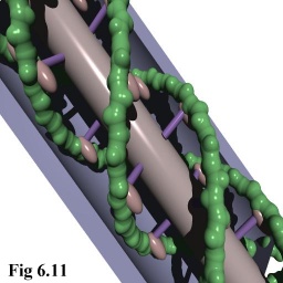
- as 'povray' ray tracer files (cf. Fig. 6.11).
 In addition, the raw scene descriptions were able to be
directly viewed using the 3-D model viewer described
below.
This modeller was used to create static models for the
nanoscale simulator (see Fig. 6.4 and 6.5) as well as the
basis models used in the 'Virtual Electron Microscopy'
described in later chapters.
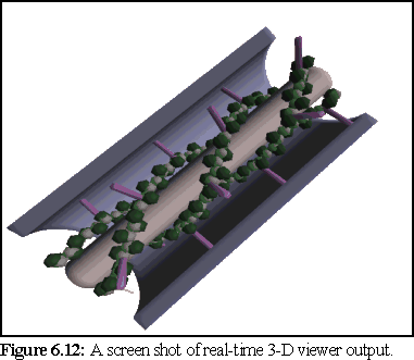
3-D Data Model Viewer
This was a 3-D viewing utility that read in the same mathematical object descriptions as used by the data
creation/conversion utility described above, and allowed the user to view them in real time, changing
viewpoint and perspective continuously when desired. But images from the 3-D viewer are not of as a
high a quality as those from the ray-tracer, because there is no anti-aliasing and smooth surfaces are not
perfectly represented as the viewer uses polygons (Fig. 6.12 below).

The real-time viewer used the SGI 'GL' library for fast rendering, and benefited from a number of
optimisations available on SGI machines, such as fast polygon pipelining. Elements of this program
were later incorporated directly into the nanoscale simulator.
1. Booch, G., Object-Oriented Analysis and Design (2nd Ed), (1994) Addison Wesley,
Menlo Park, California
2. refer any standard microtubule text. Original paper; Allen C & Borisy GG (1974)
Structural polarity and directional growth of microtubules of Chlamydomonas flagella, J.
Mol. Biol, Vol 90 pp 381-402
3. Dr. Damian Conway, Dept Computer Science and Software Engineering, Monash
University, Melbourne, Australia - personal communication.
4. Oosawa, F. & Asakura, S., op. cit.
 The polymer is responsible for moving and rotating its constituent monomers
in an orderly manner, maintaining each monomer in position relative to its
neighbours. Polymers must be able to gain and shed monomers, and be able to
merge with other polymers when required.
 The amount of data necessary to describe the behaviour of a protein monomer are far greater than can
be reasonably entered at the command line. As a result, small text files that can be written by human
users, are used instead (see 'Appendix C; Protein Dynamic Description Files' for a full language
description.)
 An
addition to the functionality of the program is the
ability to
define starting positions for the monomers.
Among
other benefits, this allows simulation of diffusion
from high-concentration regions to low-concentration regions. An obvious extension of this procedure
would be to allow complete simulation states, including linked polymers, to be read in as starting
conditions, but this has not yet been completed.


 In addition, the raw scene descriptions were able to be
directly viewed using the 3-D model viewer described
below.