Chapter 7:
Modelling Simple Structures: Actin
E lineis fit robur
(Strength comes from cords.)
_____________- anon
Index |
Last Chapter |
Next Chapter |

|
Chapter 7:Modelling Simple Structures: Actin
E lineis fit robur |

|
Actin is a common cytoskeletal protein that has been studied in great detail (see Chapter 2). It forms long, filamentous strands that are extremely common in all eukaryotic cells. It is particularly common in muscle tissue where, together with the protein myosin, it provides the mechanical forces required for muscle action (1).
This chapter looks at how the nanosim program can be used to simulate the self-assembly of actin. It examines the existing theory and experimental evidence, and shows how this can be processed to produce a behavioural model for a single actin monomer. It then describes the use of the simulator to model actin self-assembly, and reviews the program's results, comparing them with other experimental evidence.
Individual actin proteins in the unbound state are known as g-actin ("globular" actin), while actin bound within an actin strand is known as f-actin ("filamentous" actin). Actin can self-assemble in vitro, and has the property that both assembly and disassembly occur at a faster rate at one end of a filament, called the "plus" end, than at the other end of a filament, the "minus" end (Fig. 7.1) (2).
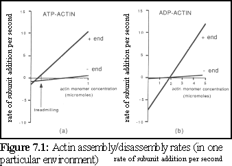
This difference in assembly and disassembly rates at either end can lead, at appropriate concentrations, to a process known as treadmilling, where a particular filament may be growing at one end while shrinking at the other.
A further complication is that, in common with many self-assembling proteins, actin dephosphorylates or hydrolyses when it binds. Phosphorylated actin has a bound adenosine 5' tri-phosphate molecule (ATP), a common energy-providing molecule used in a large number of cellular processes. This ATP molecule makes the actin protein far more likely to bind to other actin proteins. Some time after being bound, in a process that is not yet fully understood, the bound ATP molecule hydrolyses, losing a phosphate ion and becoming the less energetic adenosine 5' di-phosphate (ADP). This in turn causes the actin protein to become less securely bound.
It has been established that actin filaments usually terminate with phosphorylated ATP-actin, but whether the individual molecule dephosphorylates over time, or upon the addition of another actin molecule, is not yet completely established (a similar process, and a similar debate, occur as regards the tubulin protein examined in Chapter 8).
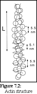
The structure of actin has been extensively studied using electron microscopy and image analysis and, despite many experimental difficulties, the nature of actin filaments is now well understood (3). It can be considered as a long two-stranded helix with a repeating length of approximately 36- 40 nm (the length 'L' in Fig. 7.2 (4)).
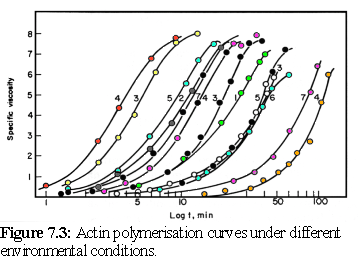
The assembly of actin is one of the finest examples of Oosawa's model of protein polymerisation in action, closely fitting the mathematical predictions made by the model (5) (cf Chapter 5). Oosawa's model predicts that the form of the polymerisation curve (a graph of the amount of the actin bound in filaments, as opposed to unbound, over time) will be the same for different environmental conditions, differing only in the rate that the reaction proceeds. Measurement of polymerisation is usually done via the viscosity of the solution, and results for the polymerisation of actin can be shown to have the same shape when plotted against logarithmic time, being simply offset by different amounts depending on whether the environmental conditions favoured rapid or slow polymerisation (Fig. 7.3) (6) :
Another prediction of Oosawa's theory is that the length distribution of actin filaments is initially a Poisson distribution at the start of polymerisation, moving to an exponential distribution when a solution has reached steady state. This is confirmed by painstaking experimental studies that have catalogued the length of actin filaments, and have found the expected exponential distribution (Fig.7.4) (7), (8):

These theoretical details, in conjunction with the wealth of experimental data, make actin an excellent candidate for trialing the nanosimulator, to see whether it reproduces correctly the behaviour of this relatively simple self-assembling protein. Actin has been previously simulated mathematically with good results, and a number of sophisticated models (including those modelling actin-associated proteins) have been developed (9), (10), (11). As far as the author is aware however the computational technique of simulating large numbers of individual actin monomers as described below is new.
Experimental studies of actin have provided accurate details of the assembly and disassembly rates of the growing filament ends. To test the simulation, an arbitrary in vitro environment is chosen for which good experimental evidence is available. The current simulation uses data from Pollard (12), who used a standard experimental environment conducive to filament growth, at 37C, and obtained the following figures (also used in figure 7.1):
| ATP-Actin | ADP-Actin | |||
| + end | - end | + end | - end | |
| kon (M-1s-1) | 11.6 | 1.3 | 3.8 | 0.16 |
| koff (s-1) | 1.4 | 0.8 | 7.2 | 0.27 |
Table 7.1 Actin association and disassociation rates (13)
Some interesting features of these figures deserve note. First, although ATP-actin is the most active and inclined to bind, it is obviously possible at higher concentrations (i.e. around the 2 M level and above) for ADP-actin to polymerise into filaments. Second, although ATP-actin is generally more likely to bind and less likely to break away than ADP-actin, in a curious inversion ADP-actin is less likely to break away from the slow-growth, "-" end of the filament.
 Using these figures, a .pddf file (the "protein dynamic
description file" used by the nanoscale simulation
program) was constructed, that uses a four-state model
for actin (Fig. 7.5):
This represents the presumed cycle of binding, dephosphorylation, unbinding, and rephosphorylation.
(Nb Figure 7.5 does not show the less common path whereby an unbound ADP-actin monomer binds immediately to a filament without rephosphorylation, although this is included in the model.)
Rephosphorylation requires an energy input into the system, and can occur when free unbound ATP replaces the phosphate-depleted ADP of a free actin protein. This occurs within the cell, and can be simulated in vitro simply by providing free molecules of unattached ATP.
Adapting the experimental figures of Table 7.1 for the simulator requires some further work. The .pddf files require binding and breaking values on an individual protein basis, rather than for the entire filament.
Deriving these from the off-rates is quite straight forward; we can use the figures from Table 7.1 directly, modifying them depending on the time step of the simulation.. For example, if the simulation uses a 100 s time step, then the ATP-actin + end off-rate of 1.4 actin molecules per second becomes .00014 actin molecules per 100 s time step.
Deriving on-rates is more complex. In order to derive these parameters, the number of interactions per second of a simulated actin protein must be determined, by running the nanosimulator in test mode. In this case, using a 100 s time step, the number of collisions of an actin protein in a 1 M solution is found to be 4050/s. The kon figures in Table 7.1, divided by this result, give the interaction probability for a single collision.
These results give us Table 7.2, in a form suitable for inclusion in our .pddf file:
| ATP-Actin | ADP-Actin | |||
| + end | - end | + end | - end | |
| p(bind)/collision | 0.00228 | 0.00033 | 0.00095 | 0.0000395 |
| P(break/100s) | 0.0001 | 0.00008 | 0.00072 | 0.000027 |
Table 7.2 Actin association and disassociation probabilities
This is graphically summarised in Fig. 7.6 and Fig. 7.7:
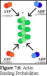
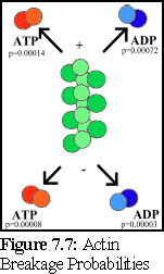
An important point to note is that it is not possible to distinguish, on the basis of the experimental evidence available, differences in binding rates depending on the state of the actin protein already bound at the tip of the filament (hence the filament is shown as uniformly green above). Although it might be suspected that such differences exist (and if they do, they can be modelled using the simulator), this particular .pddf model does not explicitly include them.
A complication arises with handling multiple breakages. For larger structures, where a protein is bound by a large number of other links, the ad hoc heuristic mentioned in Chapter 5 seems to work reasonably well (setting the overall breakage probability equal to the smallest single link breakage probability, lowered further by an order of magnitude for each extra link). But actin bound internally within a filament is linked only to two other molecules in this model (although some more recent models hypothesise that in fact links to four other actin proteins are involved (14), see also the nucleation problem below). It is an experimentally observed fact that internally bound actin very rarely, if ever, breaks away. In order to model this, when simulating actin the program is run with a special option specifying that multiple links never break.
A well observed feature of in vitro actin polymerisation is the lag phase that occurs prior to a rapid polymerisation phase (15). This lag phase is due to the instability of filaments when they are first assembling; until they reach a certain size (probably about three molecules, in the case of actin) the filament is more likely to fall apart than to grow. Once above this critical size, the filament tends to grow strongly. As more and more filaments make it over this initial barrier, polymerisation builds up speed. Added evidence that this is the reason for the lag phase lies in the observation that the lag phase can be avoided altogether if the solution is initially seeded with fragments of filamentous actin (16).
There are a number of ways this can be handled in the program. Ideally, this behaviour would grow naturally out of the binding and breaking values of the monomers. This is possible in the case of actin if the model is extended to include monomer links beyond the nearest neighbour. Unfortunately this leads into the difficulty in modelling breakages from multiple links, with the result that the breakage model chosen has a very significant impact on the nucleation lag time; in effect the user can implicitly set the lag time simply by choosing an appropriate breakage model.
Given this limitation, the current simulation was set to use a very simple model, with only neighbour-to-neighbour links, and to set the nucleation probability explicitly, by restricting the initial interaction of free actin to occur only between free ATP-actin monomers, and then with only a relatively low probability (less than for combining with a bound filament).
This same approach, of artificially restricting initial nucleation, is used widely later on in the thesis, due to this difficulty of modelling breakage rates for multiply bound proteins. It may be a promising area for future extension of the program however (see "Future Directions" in Chapter 10).
This particular .pddf file uses an 'ATP cap' model for dephosphorylation; i.e. an ATP actin monomer dephosphorylates only when it is bound to the '+' binding site. This implies that actin binding to the '+' end of a filament stays in the ATP state, while the monomer to which it binds dephosphorylates, and that an ATP actin monomer binding to the '-' end of a filament immediately dephosphorylates. A more exact model would probably include a timed decay between these states, but in the absence of experimental evidence the simpler model is used. The simulator can model this type of timed decay; for example a timed decay is often used to describe the rephosphorylation of dimers when an external source of energy is available.
The following is the .pddf file for actin assembly, based on the figures obtained in the
preceding section. As explained in Appendix C, ".pddf files", lines starting with the '#'
character are comments that are ignored by the program.
---------------------------------------------------------------------------------------------------------------
# Modelling actin assembly
#
#  figures derived from T.D. Pollard, J.Cell.Biol 1986 103, 2747-2754
#

Model Actin
{
   # model the geometry as a double sphere - distance in nm, colours as hex RGB

    Sphere centre    1.6 <-.5,-.5,0> 0x66CC66
    Sphere side      1.0 <0,-2.5,-1> 0x66CC66

   #site   name       []

    site   top      <0,0,1.5> <0,0,1> 205.714   # a link site, direction same as position
    site   bottom   <0,0,-1.5> <0,0,-1>

   #state   name    [optional colour details]

    State ATPunbound

    State ATPbound      # a new state, with no physical changes
                        # colours as RGB values in hex

        colour centre = 0xCCFFCC
        colour side   = 0xCCFFCC

    State ADPbound      # a new state, with a colour change
        colour centre = 0xAAAA00
        colour side   = 0xAAAA00

    State ADPunbound    # another new state with no physical changes
        colour centre = 0x999900
        colour side   = 0x999900

    # The event list is all of the form:
    # Event: link { A B } | break | random (chance / cycle)
    #         StateA -> StateB


    Event  bind { bottom top }                  # bottom link causes dimer to become
                                                # part of ATP "cap"
            ATPunbound -> ATPbound

    Event  bind { top bottom }                  # top link causes dimer to become
                                                # dephosphorylated
            ATPunbound -> ADPbound

    Event  bind { top bottom }                  # bottom link causes dimer to become
                                                # susceptible to dephosphorylation
            ATPbound -> ADPbound

    Event  bind { bottom top }                  # ADP actin *can* bind - it's just
                                                # not as likely.
            ADPunbound -> ADPbound

    Event  bind { top bottom }                  # ADP actin *can* bind - it's just
                                                # not as likely.
            ADPunbound -> ADPbound

    Event  break { }                        	   # if the top link is broken,
                                                #     object becomes "unbound" with
            ATPbound -> ATPunbound              #     no change in phosphorylation

    Event  break { }                        	  # if the top link is broken,

            ADPbound -> ADPunbound


    Event  random 0.00001                   	# a chance of "unbound" GDP dimer becoming
                                             # phosphorylated; avg = once every 100 seconds
            ADPunbound -> ATPunbound

}


# Specify links and states, and give their binding and breaking chance.
# links are transitive.
#
# nb.  All these rely on a time constant of 100 microseconds...
#
# nb II : The 'break' coefficient of unbound objects is, of course, meaningless...
#         since they're not bound, they have nothing to break from... hence the '0's.
#         Also, some of these should never occur, because of the "instant
#         dephosphorylation" model currently used.
#
# nb III : Estimation of free -> free binding links.  This is unknown - as a first
#          approximation, use a low initial nucleation probability...
#


#ATP - ATP binding
# n.b.: current model never has 2 bound ATPs together; hence break(1) if it does.
# also; bottom state should never happen for the same reason.

Binding Actin top ATPunbound to Actin bottom ATPunbound  = bind(0.000001) break(1)
Binding Actin top ATPunbound to Actin bottom ATPbound    = bind(0.00014) break(1)
Binding Actin top ATPbound   to Actin bottom ATPunbound  = bind(0.00288) break(1)
Binding Actin top ATPbound   to Actin bottom ATPbound    = bind(0) break(1)

# ATP - ADP bindings
Binding Actin top ATPunbound to Actin bottom ADPunbound = bind(0) break(1)
Binding Actin top ATPunbound to Actin bottom ADPbound   = bind(0.00014) break(1)
Binding Actin top ATPbound   to Actin bottom ADPunbound = bind(0.00095) break(1)
Binding Actin top ATPbound   to Actin bottom ADPbound   = bind(0.00014) break(0.00008)

Binding Actin top ADPunbound to Actin bottom ATPunbound = bind(0)  break(1)
Binding Actin top ADPunbound to Actin bottom ATPbound   = bind(0.00004) break(1)
Binding Actin top ADPbound   to Actin bottom ATPunbound = bind(0.00228) break(1)
Binding Actin top ADPbound   to Actin bottom ATPbound   = bind(0.00228) break(0.00014)

# ADP - ADP bindings

Binding Actin top ADPunbound to Actin bottom ADPunbound = bind(0)  break(1)
Binding Actin top ADPunbound to Actin bottom ADPbound   = bind(0.00004) break(1)
Binding Actin top ADPbound   to Actin bottom ADPunbound = bind(0.00095) break(1)
Binding Actin top ADPbound   to Actin bottom ADPbound   = bind(0.00095)  break(.00008)


# some environment constants

Temperature 310  	# kelvin - physiological temperature
Viscosity   0.62 	# approximate viscosity for water at 37 degrees Celsius
			        # (nb: .69 cP would be more accurate)
TimeScale   100   	# microseconds per program cycle - this is at the very top of the
			        # allowable range, so as to get long results; it would be better at 10
			        # microseconds
			        # (nb. This would require recalculating the number of collisions/second)

# Finally, specify the mix of molecules in solution.

Mix Actin 100%		# (We're using only actin in this simulation)
Using the figures from the previous section, the simulator was run under the following conditions:
simulate time period: 10 seconds
volume: 512nm x 512nm x 512nm; i.e.� m cubed
molarity: 2.5 M.-
timestep: 100 s timesteps
temperature: Temperature 310 (physiological temperature)
viscosity: 0.62 cP (approx viscosity of water at 310 K (17))
The following sections illustrate results from this (single) run of the program. Note that a relatively high molarity (2.5 M) was used so that the simulation would produce useful results within 10 simulated seconds. Ths required approximately a week of computer time on an SGI O2 machine (18).
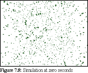
(These images were rendered in Povray, with perspective.)
At the beginning of the simulation (Fig.7.8), there are only free monomers in solution:
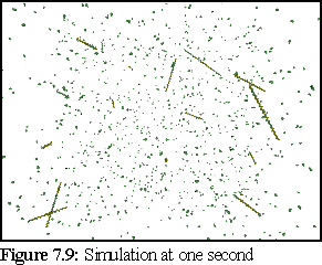
After a simulated second, a number of short filaments have started to grow (Fig. 7.9). At the end of each filament appears a green monomer, representing the ATP cap of the filament. (This may not be visible at the scale of this picture.)
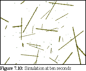
After ten virtual seconds, the simulation has
used up almost all the free monomers, and the
filaments are starting to lose monomers, which
will slowly rephosphorylate as the solution
enters an equilibrium state (Fig. 7.10).
One of the features of the program's logging facility is the ability to save data on a single filament, or a small set of filaments, and thus track their growth. This was done in the current simulation for the first filament, which was created between 60 and 80 (virtual) ms into the program run (since the concentration was so high), and remained in existence for the life of the simulation. Figure 7.11 shows that the time at which the bulk of free ATP-actin was used must have been around about the (simulated) 2� second mark. (Nb the graph starts at '6' since this is the size the filament grew to in the 20 ms pause between creation and the first logging point.)
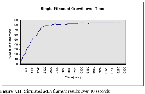
It is instructive to compare the growth of this single filament with the
predictions of table 7.1. In theory, the filament should grow at a rate of 30 monomers/second
(remembering that addition occurs at both ends). During the rapid growth phase (the first 1.5
seconds above) the filament grows at greater than the expected rate, adding 53 monomers in the
first 1.5 seconds, or 35 monomers/second. Using the binomial approximation that the standard
deviation is approximately equal to the square root of the mean (![]() ), we find the standard
deviation as 5.48, so this faster growth is not particularly remarkable. But the most likely
explanation lies in the erroneously low viscosity of 0.62 cP rather than 0.69cP - if the time scale is
multiplied by 1.11 (as a first approximation - the real variation is somewhat more complex due to
the program not scaling linearly) to adjust for this, the on rate is found to be 31.5
monomers/second, almost exactly as predicted. A further possible factor is the increased motility
of small fragments leads to a slightly larger number of collisions than when the fragment is larger.
), we find the standard
deviation as 5.48, so this faster growth is not particularly remarkable. But the most likely
explanation lies in the erroneously low viscosity of 0.62 cP rather than 0.69cP - if the time scale is
multiplied by 1.11 (as a first approximation - the real variation is somewhat more complex due to
the program not scaling linearly) to adjust for this, the on rate is found to be 31.5
monomers/second, almost exactly as predicted. A further possible factor is the increased motility
of small fragments leads to a slightly larger number of collisions than when the fragment is larger.
Tracking a significantly larger population of filaments however would give a useful check on the system's accuracy, as the average growth rate should still be 30 monomers/second.
After this growth period, with the quantity of free actin greatly reduced, we expect that the filament will slowly shrink. But unless it loses its ATP cap this shrinkage will be quite slow, on the order of one monomer every four seconds (from the '-' end) and 0.8 monomers a second from the '+' end (cf table 7.1).
Figure 7.12 shows the amount of filamentous actin over time. Since the concentration is high and the volume small, the sample reaches saturation more swiftly than a traditional experimental run in which the polymerisation might curve might be observed over minutes or even hours (as opposed to ten seconds in this run) but the form of the polymerisation curve, as predicted by Oosawa's model, is the same as in those longer runs (cf Fig. 7.3 for experimental results).
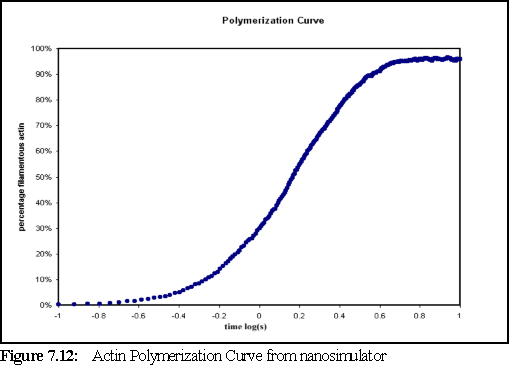
Figure 7.12 shows us that almost all the monomeric actin has been polymerised by five seconds. However, the sample has not yet reached steady state, since ADP-actin has been set (in the .pddf file) to rephosphorylate to ATP-actin, on average, once every 100 seconds. Tracking the state of the monomers, shows that the amount of free ATP-actin passed the theoretical critical concentration (the concentration at which filaments are stable, but do not grow) of 0.18 M (115 monomers) at around four seconds. At the end of the simulation, at ten seconds, there are 65 free-ATP actin monomers (equivalent to 0.1 M) still remaining, and the simulation appears to be close to steady state. The smaller than expected number of free monomers may indicate an over estimation of bonding strength in the model.
Another interesting result is the size distribution of filaments. Unfortunately, due to the small number of filaments (less than thirty) there is significant noise in the data. Figure 7.13 shows the change in the size distribution over the first five seconds (significant change does not occur over the final five seconds of the simulation). The chart shows the number of filaments in a given size range at a particular time (i.e. in the chart below there are five filaments of size 16-24 monomers, at time 0.5 seconds - and this is represented by the dark purple peak below).
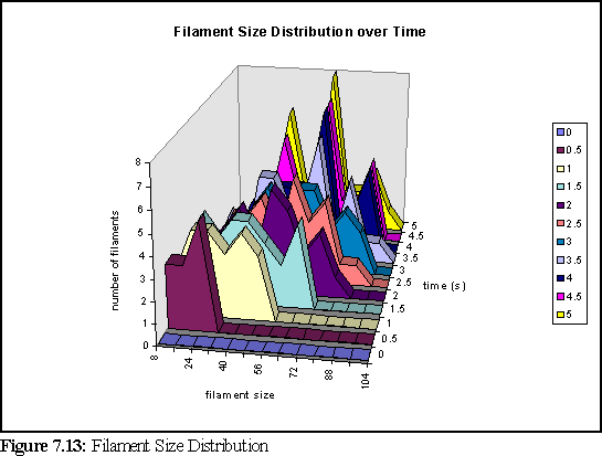
To further clarify the above chart, Fig. 7.14 and 7.15 show the filament size distributions at one second and at five seconds.
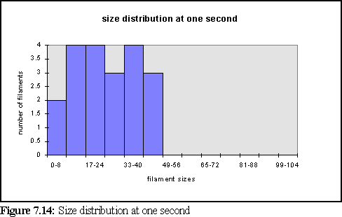
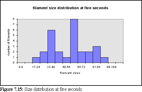
With a certain amount of imagination these might be viewed as the expected Poisson distributions (19) with a great deal of noise. However strictly all that can be said is that at this scale of simulation, with only dozens of filaments, it is not possible to accurately specify the size distribution of filaments, and that a larger simulation would need to be run on a faster computer to properly study this feature. It is also expected that the simulation would have to be run for longer, to reach steady state, until it could reproduce the experimental results of figure 7.4 .
This simulation of actin shows that the nanoscale simulator is capable of modelling many of the characteristics of actin polymerisation during the initial growth phase. The simulator demonstrated the characteristic polymerisation curve, was able to track the initial growth phase of individual filaments, and obtained various statistics and information about the distribution of filaments during growth.
Longer runs in the future should provide even more detailed models of the long-term behaviour of actin. It has not been possible (yet) to run the simulation for long enough to observe features such as the full cycle of actin filament growth, collapse and possible rescue, or the steady state rephosphorylation of ADP-actin into ATP-actin to maintain the growth/collapse cycle. However the ability of the program to run for an extended period of time (in the case of the simulation here, one week) indicates that longer and larger simulation runs should be quite practical in the future, especially given the continuing improvements in computer hardware.
Index |
Last Chapter |
Next Chapter |
1. For further background see Amos, L.A. and Amos, B.A.(1991), Molecules of the Cytoskeleton, Macmillan, London, Chapter 3 pp 42-55
2. Image from ibid, p 51
3. Engleman, E.H. (1985) The structure of the actin thin filament. J.Muscle Res. & Cell Motil., Vol 6, pp 129-151
4. Image from Amos, op. cit., p43
5. Oosawa, F. and Asakura, S. (1975), Thermodynamics of the Polymerisation of Protein, Academic Press, London.
6. Figure ibid p50
7. Kawamura, M., and Maruyama, K. (1970), Electron microscopic particle length of F-actin polymerised in vitro, J. Biochem, Vol 67, pp 437-457
8. Kawamura, M., and Maruyama, K. (1972), A further study of electron microscopic particle length of F-actin polymerised in vitro, J. Biochem, Vol 72, 179-188
9. Civelekoglu, G., and Edelstein-Keshet, L., (1994), Modelling the dynamics of f-actin in the cell, Bull. Math. Biol., Vol 56, No 4., pp 587-616
10. Sherratt, J.A. and Lewis, J., (1993), Stress induced alignment of actin filaments and the mechanism of cytogel, Bull. Math. Biol., Vol 55, pp 637-654
11. Alt. W., (1987) Mathematical models in actin-myosin interaction, in Fortshiritte der Zoology, Nature and Funciton of Cytoskeletal Proteins in Motility and Transport, Band 34, K.E. Wohlfarth-Bottermann(Ed)., pp 219-230, Stuttgart: Gustav Fisher Verlag, cited Civelekoglu op. cit.
12. Pollard, T.D. (1986), Rate constants for the reactions of ATP- and ADP- actin with the ends of actin filaments., J. Cell Biol., Vol 103, pp 2747-2754
13. Ibid
14. Amos, L.A. and Amos, B.A. (1991), Molecules of the Cytoskeleton, Macmillan, London, Chapter 3, p52
15. Oosawa, F. and Asakura, S. (1975), Thermodynamics of the Polymerisation of Protein, Academic Press, London.
16. Ibid.
17. This figure, which was widely used by the author, was read off the graph of water
viscosity that appears in Atkins (op. cit.) on p834. A later calculation by the author using
the empirical equation (Atkins, footnote to Appendix C table 24.3):
![]()
gives the more exact value 0.69 cP. The effect of this adjustment is to make water more viscous; hence the movement of molecules in simulations using the smaller figure is slightly faster than is strictly correct.
18. Note that all times mentioned in seconds during this and subsequent chapters refer to simulated seconds - the actual simulation times on the computer were all on the order of hours or days.
19. Oosawa, F. and Asakura. S. op. cit. p46